Numerical Methods

#|echo: false
import numpy as np
import matplotlib.pyplot as plt
#plt.ion()

Numerical differentiation

While differentiation is easier for humans than Integration it is the other way around for computers. Since integration is basically summation, numerical differentiation builds upon small differnences

Method of finite differences

Finite differences are used in many numerical techniques. Sometimes there is no expression for the function, only its values on a grid. The idea is to use Taylor series expansion, backwards and forwards, with different step sizes, to obtain the derivative of the desired order (with less or more precision):

\[ f(x+h) = f(x) + hf'(x) + \frac{h^2}{2!}f''(x)+\frac{h³}{3!}f'''(x)+ … \]

\[ f(x+h) = \sum_{n=1}^{N} \frac{h^n}{n!}f^{n}(x) \]

\[ f(x-h) = \sum_{n=2}^{N} \frac{h^n}{n!}f^n(x)- \frac{h^{n+1}}{(n+1)!}f^{n+1}(x) \] \[ f(x+2h) = \sum_{n=0}^{N} \frac{2h^n}{2n!}f^n(x) \] \[ f(x-2h) = \sum_{n=2}^{N} \frac{2h^n}{n!}f^n(x)- \frac{2h^{n+1}}{(n+1)!}f^{n+1}(x) \\ \]

Primary approximation of central differencials

\[ f'(x) = \frac{f(x+h)-f(x-h)}{2h} +O(h²) \\ \]

\[ f''(x) = \frac{f(x+h)-2f(x)+f(x-h)}{h²} + O(h^2) \\ \]

\[ f'''(x) = \frac{f(x+2h)-2f(x+h)+2f(x-h)-f(x-2h)}{2h} +O(h²) \\ \]

\[ f^{(4)}(x) = \frac{f(x+2h)-4f(x+h)+6f(x)-4f(x-h)+f(x-2h)}{h⁴} + O(h^2) \\ \]

\[ eq:\\ \]

\[ h^4 f^{(4)}(x) +O(h^6)= f(x+2h)-4f(x+h)+6f(x)-4f(x-h)+f(x-2h) \]

By adding and subtracting the forward and backward expansions, some terms can be eliminated. The different derivatives are thus obtained, with precision up to a certain order.

In the following example, even or odd terms are eliminated in the order of the derivatives.


f = lambda x : np.log2(x)
df = lambda x : 1/x
dff = lambda x : -1/x**2

x = np.linspace(1,60,60)

#plt.close()
plt.plot(x,f(x),x,df(x),x,dff(x))
plt.title("Function position as a function of time \n $pos =  log(time)$")
plt.xlabel("time")
plt.ylabel("position | speed | acceleration ")
plt.show()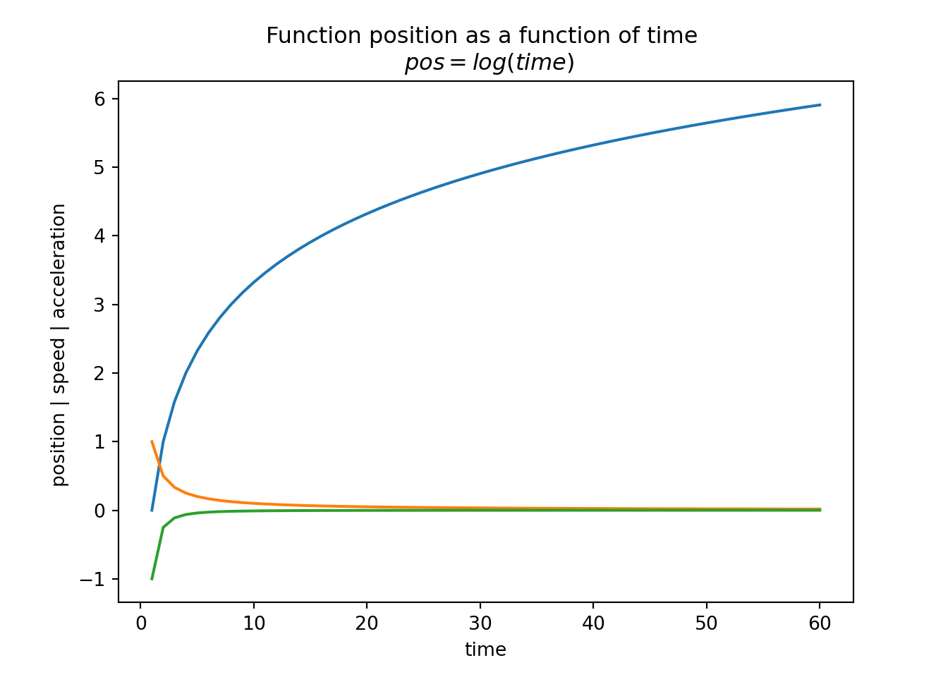

a = [(f(x+0.5)-f(x))/0.5 for x in x]
a2 = [(f(x+0.5)-f(x-0.5))/2*0.5 for x in x]
a4 = [(-f(x+2*0.5)+8*f(x+0.5)-8*f(x-0.5)+f(x-2*0.5))/12*0.5 for x in x]
#plt.close()

<string>:1: RuntimeWarning: divide by zero encountered in log2

plt.plot(x,df(x),x,a,x,a2, x,a4)
plt.title("approximation of acceleration function df")
plt.show()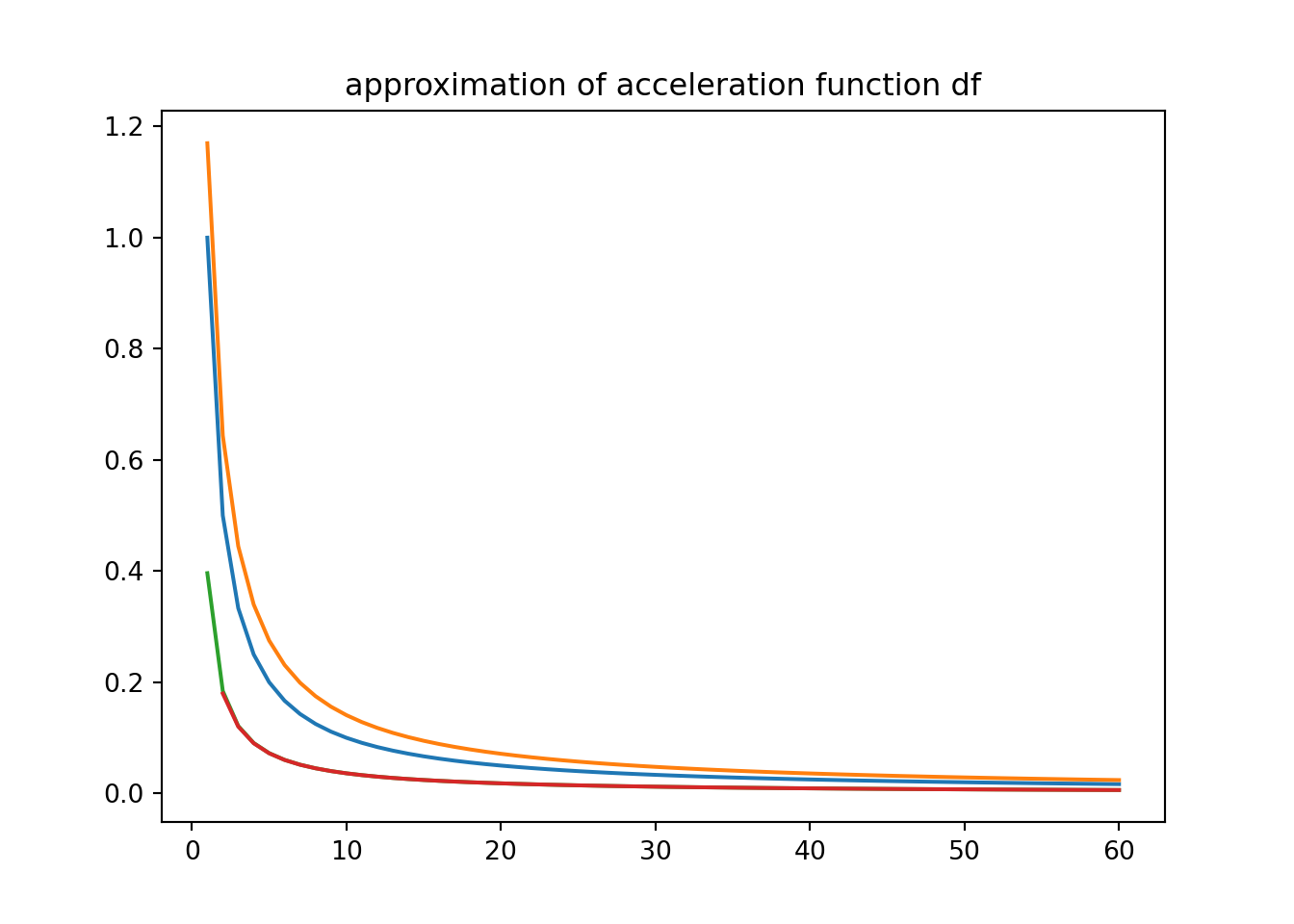

f = lambda x: np.sin(x)

domain = np.arange(0,3*np.pi,0.01)

N_inter = 100

h = (max(domain)-min(domain)) / N_inter


y = [f(x) for x in domain]


# first derivative
## forwards
f1f = lambda f,x,h : (-3*f(x[0])+4*f(x[1])-f(x[2])) / 2*h 
## backwards
f1b = lambda f,x,h : (-3*f(x[0])+4*f(x[-1])-f(x[-2])) / 2*h 
# second Derivative forward
f2f = lambda f,x,h : (f(x[0])-2*f(x[1])+f(x[2])) / h**2
# second Derivative backward
f2f = lambda f,x,h : (f(x[0])-2*f(x[1])+f(x[2])) / h**2


## forwards
f1f = lambda f,x,h : (-3*f(x)+4*f(x+h)-f(x+2*h)) / 2*h 
## backwards
f1b = lambda f,x,h : (-3*f(x[0])+4*f(x[-1])-f(x[-2])) / 2*h 
# second Derivative forward
f2f = lambda f,x,h : (f(x[0])-2*f(x[1])+f(x[2])) / h**2
# second Derivative backward
f2f = lambda f,x,h : (f(x[0])-2*f(x[1])+f(x[2])) / h**2

y[1:-1]

[0.009999833334166664, 0.01999866669333308, 0.02999550020249566, 0.03998933418663416, 0.04997916927067833, 0.059964006479444595, 0.06994284733753277, 0.0799146939691727, 0.08987854919801104, 0.09983341664682815, 0.10977830083717481, 0.11971220728891936, 0.12963414261969486, 0.1395431146442365, 0.14943813247359922, 0.15931820661424598, 0.16918234906699603, 0.17902957342582418, 0.18885889497650057, 0.19866933079506122, 0.20845989984609956, 0.21822962308086932, 0.2279775235351884, 0.23770262642713458, 0.24740395925452294, 0.2570805518921551, 0.26673143668883115, 0.27635564856411376, 0.28595222510483553, 0.29552020666133955, 0.3050586364434435, 0.31456656061611776, 0.32404302839486837, 0.3334870921408144, 0.3428978074554514, 0.35227423327508994, 0.361615431964962, 0.3709204694129827, 0.3801884151231614, 0.3894183423086505, 0.39860932798442295, 0.40776045305957015, 0.41687080242921076, 0.4259394650659996, 0.43496553411123023, 0.4439481069655198, 0.45288628537906833, 0.4617791755414829, 0.470625888171158, 0.479425538604203, 0.4881772468829075, 0.49688013784373675, 0.5055333412048469, 0.5141359916531132, 0.5226872289306592, 0.5311861979208834, 0.5396320487339693, 0.5480239367918736, 0.5563610229127838, 0.5646424733950354, 0.5728674601004813, 0.5810351605373051, 0.5891447579422695, 0.5971954413623921, 0.6051864057360395, 0.6131168519734338, 0.6209859870365597, 0.6287930240184686, 0.636537182221968, 0.6442176872376911, 0.6518337710215366, 0.6593846719714731, 0.6668696350036979, 0.674287911628145, 0.6816387600233341, 0.6889214451105513, 0.6961352386273567, 0.7032794192004101, 0.7103532724176078, 0.7173560908995228, 0.7242871743701426, 0.7311458297268959, 0.7379313711099628, 0.7446431199708593, 0.7512804051402927, 0.757842562895277, 0.7643289370255051, 0.7707388788989693, 0.7770717475268238, 0.7833269096274834, 0.7895037396899505, 0.795601620036366, 0.8016199408837772, 0.8075581004051143, 0.8134155047893737, 0.8191915683009983, 0.8248857133384501, 0.8304973704919705, 0.8360259786005205, 0.8414709848078965, 0.8468318446180152, 0.852108021949363, 0.8572989891886034, 0.8624042272433384, 0.867423225594017, 0.8723554823449863, 0.8772005042746817, 0.8819578068849475, 0.8866269144494873, 0.8912073600614354, 0.8956986856800476, 0.9001004421765051, 0.904412189378826, 0.9086334961158833, 0.9127639402605211, 0.9168031087717669, 0.9207505977361357, 0.9246060124080203, 0.9283689672491666, 0.9320390859672263, 0.9356160015533859, 0.9390993563190676, 0.9424888019316975, 0.945783999449539, 0.9489846193555862, 0.9520903415905158, 0.9551008555846923, 0.9580158602892249, 0.9608350642060727, 0.963558185417193, 0.966184951612734, 0.9687151001182652, 0.9711483779210446, 0.9734845416953194, 0.9757233578266591, 0.9778646024353163, 0.9799080613986142, 0.9818535303723598, 0.9837008148112766, 0.9854497299884603, 0.9871001010138504, 0.9886517628517197, 0.9901045603371778, 0.9914583481916864, 0.9927129910375885, 0.9938683634116449, 0.9949243497775809, 0.99588084453764, 0.9967377520431434, 0.9974949866040544, 0.9981524724975481, 0.998710143975583, 0.999167945271476, 0.9995258306054791, 0.999783764189357, 0.9999417202299663, 0.9999996829318346, 0.9999576464987401, 0.9998156151342908, 0.9995736030415051, 0.9992316344213905, 0.998789743470524, 0.9982479743776325, 0.9976063813191737, 0.9968650284539189, 0.9960239899165367, 0.9950833498101802, 0.994043202198076, 0.9929036510941185, 0.9916648104524686, 0.990326804156158, 0.9888897660047015, 0.9873538397007164, 0.9857191788355535, 0.9839859468739369, 0.9821543171376185, 0.9802244727880455, 0.9781966068080447, 0.9760709219825242, 0.9738476308781951, 0.9715269558223153, 0.9691091288804563, 0.9665943918332975, 0.9639829961524481, 0.9612752029752999, 0.9584712830789142, 0.955571516852944, 0.9525761942715953, 0.9494856148646305, 0.9463000876874145, 0.9430199312900105, 0.9396454736853249, 0.9361770523163061, 0.9326150140222005, 0.9289597150038693, 0.9252115207881683, 0.9213708061913954, 0.9174379552818098, 0.9134133613412252, 0.9092974268256817, 0.9050905633252009, 0.9007931915226273, 0.8964057411515598, 0.8919286509533796, 0.8873623686333755, 0.8827073508159741, 0.8779640629990781, 0.8731329795075164, 0.8682145834456126, 0.8632093666488737, 0.8581178296348089, 0.8529404815528762, 0.8476778401335698, 0.8423304316366457, 0.8368987907984977, 0.8313834607786831, 0.825784993105608, 0.8201039476213742, 0.814340892425796, 0.8084964038195901, 0.8025710662467472, 0.7965654722360865, 0.7904802223420048, 0.7843159250844198, 0.7780731968879212, 0.7717526620201257, 0.7653549525292536, 0.7588807081809218, 0.7523305763941707, 0.74570521217672, 0.7390052780594708, 0.7322314440302514, 0.7253843874668195, 0.7184647930691263, 0.7114733527908443, 0.7044107657701763, 0.6972777382599378, 0.6900749835569364, 0.6828032219306397, 0.675463180551151, 0.668055593416491, 0.6605812012792007, 0.6530407515722648, 0.6454349983343707, 0.6377647021345036, 0.6300306299958922, 0.6222335553193047, 0.6143742578057118, 0.6064535233783147, 0.5984721441039565, 0.5904309181139127, 0.5823306495240819, 0.5741721483545723, 0.5659562304487028, 0.5576837173914166, 0.5493554364271266, 0.5409722203769886, 0.5325349075556212, 0.5240443416872761, 0.5155013718214642, 0.5069068522480534, 0.49826164241183857, 0.4895666068265995, 0.48082261498864826, 0.47203054128988264, 0.4631912649303452, 0.45430566983030646, 0.44537464454187115, 0.4363990821601263, 0.4273798802338298, 0.418317940675659, 0.4092141696720173, 0.4000694775924195, 0.3908847788984522, 0.38166099205233167, 0.3723990394250553, 0.3630998472041683, 0.3537643453011427, 0.34439346725839, 0.33498815015590466, 0.32554933451756, 0.3160779642170538, 0.30657498638352293, 0.2970413513068324, 0.2874780123425444, 0.2778859258165868, 0.2682660509296179, 0.25861934966111083, 0.24894678667315256, 0.23924932921398243, 0.2295279470212642, 0.21978361222511694, 0.21001729925089915, 0.20022998472177053, 0.19042264736102704, 0.18059626789423291, 0.17075182895114532, 0.16089031496745576, 0.15101271208634384, 0.1411200080598672, 0.1312131921501838, 0.12129325503062975, 0.11136118868664958, 0.10141798631660186, 0.09146464223243675, 0.08150215176026912, 0.07153151114084326, 0.06155371742991315, 0.05156976839853464, 0.04158066243329049, 0.031587398436453896, 0.02159097572609596, 0.011592393936158275, 0.0015926529164868282, -0.008407247367148618, -0.01840630693305381, -0.02840352588360379, -0.03839790450523538, -0.04838844336841415, -0.058374143427580086, -0.06835400612104778, -0.0783270334708653, -0.0882922281826076, -0.09824859374510868, -0.10819513453010837, -0.11813085589181781, -0.12805476426637968, -0.13796586727122728, -0.14786317380431852, -0.15774569414324865, -0.16761244004421832, -0.17746242484086058, -0.18729466354290317, -0.19710817293466984, -0.20690197167339977, -0.21667508038737962, -0.22642652177388314, -0.236155320696897, -0.24586050428463702, -0.2555411020268312, -0.26519614587177337, -0.274824670323124, -0.28442571253646254, -0.2939983124155676, -0.30354151270842933, -0.3130543591029702, -0.322535900322479, -0.3319851882207341, -0.34140127787682095, -0.35078322768961984, -0.36013009947196856, -0.3694409585444771, -0.37871487382899804, -0.3879509179417303, -0.3971481672859602, -0.4063057021444168, -0.41542260677124626, -0.4244979694835826, -0.43353088275271773, -0.44252044329485246, -0.45146575216142315, -0.4603659148289983, -0.46922004128872713, -0.47802724613534286, -0.48678664865569937, -0.4954973729168449, -0.5041585478536115, -0.5127693073557238, -0.5213287903544065, -0.5298361409084934, -0.5382905082900177, -0.5466910470692872, -0.5550369171994238, -0.56332728410037, -0.5715613187423437, -0.5797381977287431, -0.5878571033784827, -0.5959172238077642, -0.6039177530112606, -0.6118578909427193, -0.6197368435949633, -0.6275538230792936, -0.6353080477042756, -0.6429987420539088, -0.6506251370651673, -0.6581864701049049, -0.6656819850461192, -0.6731109323435617, -0.680472569108694, -0.6877661591839738, -0.694990973216472, -0.7021462887308054, -0.7092313902013861, -0.7162455691239705, -0.7231881240865121, -0.7300583608392995, -0.7368555923643834, -0.7435791389442746, -0.750228328229919, -0.7568024953079282, -0.7633009827670734, -0.7697231407640244, -0.7760683270883323, -0.7823359072266528, -0.788525254426195, -0.7946357497573974, -0.8006667821758177, -0.8066177485832405, -0.8124880538879843, -0.8182771110644103, -0.8239843412116258, -0.8296091736113709, -0.8351510457850935, -0.8406094035501945, -0.8459837010754465, -0.8512734009355745, -0.8564779741650012, -0.8615969003107405, -0.8666296674844443, -0.8715757724135882, -0.8764347204918014, -0.8812060258283253, -0.8858892112966027, -0.8904838085819885, -0.8949893582285835, -0.8994054096851777, -0.9037315213503057, -0.9079672606164054, -0.9121122039130803, -0.9161659367494549, -0.920128053755624, -0.9239981587231879, -0.9277758646448755, -0.9314607937532425, -0.9350525775584494, -0.9385508568851079, -0.941955281908201, -0.9452655121880633, -0.9484812167044256, -0.951602073889516, -0.9546277716602164, -0.9575580074492711, -0.9603924882355434, -0.9631309305733167, -0.9657730606206388, -0.9683186141667072, -0.9707673366582883, -0.9731189832251739, -0.9753733187046665, -0.977530117665097, -0.9795891644283669, -0.9815502530915156, -0.9834131875473108, -0.9851777815038595, -0.9868438585032365, -0.9884112519391306, -0.9898798050735039, -0.991249371052267, -0.9925198129199632, -0.9936910036334645, -0.9947628260746756, -0.9957351730622453, -0.9966079473622855, -0.9973810616980933, -0.9980544387588794, -0.9986280112074989, -0.9991017216871848, -0.999475522827284, -0.999749377247994, -0.9999232575641008, -0.999997146387718, -0.9999710363300245, -0.9998449300020044, -0.9996188400141854, -0.999292788975378, -0.9988668094904142, -0.9983409441568876, -0.9977152455608933, -0.9969897762717695, -0.9961646088358407, -0.9952398257691626, -0.9942155195492713, -0.9930917926059354, -0.9918687573109126, -0.9905465359667132, -0.9891252607943698, -0.9876050739202153, -0.9859861273616704, -0.9842685830120416, -0.9824526126243325, -0.9805383977940689, -0.9785261299411385, -0.9764160102906497, -0.9742082498528091, -0.9719030694018208, -0.9695006994538088, -0.967001380243766, -0.9644053617015305, -0.9617129034267934, -0.9589242746631385, -0.9560397542711181, -0.9530596307003675, -0.9499842019607608, -0.9468137755926089, -0.9435486686359066, -0.9401892075986283, -0.9367357284240789, -0.9331885764572976, -0.9295481064105251, -0.9258146823277321, -0.9219886775482162, -0.918070474669267, -0.914060465507907, -0.9099590510617106, -0.9057666414687044, -0.9014836559663548, -0.8971105228496424, -0.8926476794282346, -0.8880955719827542, -0.8834546557201531, -0.8787253947281899, -0.8739082619290224, -0.8690037390319161, -0.8640123164850744, -0.858934493426592, -0.8537707776345433, -0.8485216854762041, -0.8431877418564168, -0.8377694801650978, -0.8322674422239013, -0.8266821782320357, -0.821014246711247, -0.8152642144499634, -0.8094326564466194, -0.8035201558521553, -0.7975273039117042, -0.791454699905466, -0.7853029510887806, -0.7790726726314031, -0.7727644875559871, -0.7663790266757844, -0.759916928531561, -0.7533788393277465, -0.7467654128678123, -0.7400773104888944, -0.7333152009956565, -0.7264797605934131, -0.7195716728205075, -0.7125916284799615, -0.7055403255703919, -0.6984184692162135, -0.6912267715971264, -0.6839659518769007, -0.6766367361314569, -0.669239857276262, -0.6617760549930369, -0.6542460756557914, -0.6466506722561834, -0.6389906043282237, -0.6312666378723208, -0.6234795452786853, -0.6156301052500863, -0.6077191027239858, -0.5997473287940438, -0.5917155806310094, -0.5836246614030073, -0.5754753801952172, -0.5672685519289686, -0.5590049972802488, -0.5506855425976376, -0.5423110198196698, -0.5338822663916443, -0.5254001251818793, -0.5168654443974288, -0.5082790774992584, -0.49964188311690244, -0.49095472496260095, -0.48221847174493154, -0.47343399708193507, -0.46460217941375737, -0.4557239019148047, -0.44680005240543, -0.4378315232631469, -0.4288192113333959, -0.4197640178398589, -0.41066684829434086, -0.4015286124062146, -0.39235022399145386, -0.38313260088125134, -0.373876664830236, -0.3645833414243013, -0.35525355998804264, -0.34588825349182883, -0.3364883584585042, -0.32705481486974064, -0.31758856607203484, -0.3080905586823781, -0.2985617424935936, -0.2890030703793611, -0.27941549819892586, -0.26979998470151617, -0.26015749143046807, -0.2504889826270749, -0.2407954251341592, -0.23107778829939224, -0.22133704387835867, -0.21157416593738504, -0.2017901307561289, -0.19198591672995502, -0.18216250427209502, -0.17232087571561025, -0.1624620152151542, -0.15258690864856114, -0.14269654351825772, -0.13279190885251674, -0.12287399510655005, -0.11294379406346737, -0.10300229873509785, -0.0930505032626889, -0.0830894028174964, -0.07311999350126308, -0.06314327224661277, -0.053160236717356125, -0.04317188520872868, -0.03317921654755682, -0.02318322999237945, -0.013184925133521251, -0.0031853017931379904, 0.006814640074770176, 0.016813900484349713, 0.026811479517893238, 0.03680637742582692, 0.04679759472668989, 0.05678413230707805, 0.06676499152155635, 0.07673917429251892, 0.08670568321000133, 0.09666352163141724, 0.10661169378122355, 0.11654920485049364, 0.1264750610964027, 0.13638826994159764, 0.14628784007345494, 0.1561727815432119, 0.1660421058649572, 0.175894826114484, 0.18572995702797787, 0.19554651510054424, 0.2053435186845546, 0.21511998808781552, 0.2248749456715337, 0.2346074159480808, 0.24431642567853773, 0.2540010039700231, 0.2636601823727784, 0.27329299497701326, 0.28289847850949296, 0.2924756724298697, 0.30202361902673236, 0.3115413635133787, 0.32102795412328977, 0.3304824422053109, 0.3399038823185127, 0.3492913323267357, 0.35864385349280037, 0.36796051057238466, 0.3772403719075444, 0.38648250951987934, 0.3956859992033308, 0.4048499206165983, 0.413973357375178, 0.42305539714299684, 0.43209513172364716, 0.44109165715120235, 0.4500440737806176, 0.4589514863776903, 0.4678130042085843, 0.4766277411288995, 0.48539481567229026, 0.49411335113860816, 0.5027824756815727, 0.5114013223959524, 0.5199690294042587, 0.5284847399429308, 0.5369476024480118, 0.545356770640302, 0.5537114036099907, 0.562010665900743, 0.5702537275932467, 0.5784397643882001, 0.5865679576887464, 0.5946374946823286, 0.6026475684219723, 0.6105973779069791, 0.618486128163024, 0.6263130303216559, 0.6340773016991814, 0.6417781658749337, 0.6494148527689112, 0.6569865987187891, 0.664492646556282, 0.6719322456828621, 0.6793046521448148, 0.6866091287076385, 0.6938449449297637, 0.7010113772355987, 0.7081077089878838, 0.7151332305593578, 0.7220872394037184, 0.7289690401258765, 0.7357779445514936, 0.7425132717958018, 0.7491743483316894, 0.7557605080570543, 0.7622710923614112, 0.7687054501917558, 0.775062938117667, 0.78134292039565, 0.787544769032711, 0.7936678638491531, 0.7997115925405982, 0.8056753507392133, 0.8115585420741488, 0.8173605782311729, 0.8230808790115055, 0.8287188723898353, 0.8342739945715234, 0.8397456900489799, 0.8451334116572173, 0.8504366206285644, 0.8556547866465439, 0.8607873878989016, 0.8658339111297899, 0.8707938516910911, 0.8756667135928826, 0.8804520095530344, 0.8851492610459383, 0.8897579983503596, 0.8942777605964088, 0.8987080958116269, 0.9030485609661848, 0.907298722017184, 0.9114581539520613, 0.9155264408310896, 0.9195031758289707, 0.9233879612755189, 0.927180408695427, 0.9308801388471136, 0.934486781760646, 0.9379999767747389, 0.9414193725728183, 0.9447446272181541, 0.9479754081880525, 0.951111392407109, 0.9541522662795148, 0.9570977257204173, 0.9599474761863261, 0.9627012327045701, 0.9653587199017918, 0.9679196720314865, 0.970383833000575, 0.9727509563950137, 0.9750208055044363, 0.977193153345823, 0.9792677826862, 0.9812444860643621, 0.9831230658116188, 0.9849033340715608, 0.9865851128188459, 0.9881682338770004, 0.989652538935238, 0.9910378795642898, 0.9923241172312475, 0.9935111233134158, 0.9945987791111761, 0.9955869758598548, 0.9964756147406006, 0.9972646068902659, 0.9979538734102932, 0.998543345374605, 0.999032963836496, 0.9994226798345279, 0.999712454397426, 0.9999022585479752, 0.9999920733059188, 0.9999818896898556, 0.999871708718139, 0.9996615414087742, 0.999351408778317, 0.998941341839772, 0.9984313815994914, 0.9978215790530743, 0.997111995180267, 0.9963027009388656, 0.9953937772576199, 0.9943853150281404, 0.9932774150958098, 0.992070188249698, 0.9907637552114835, 0.9893582466233818, 0.9878538030350801, 0.9862505748896837, 0.9845487225086711, 0.9827484160758618, 0.9808498356203995, 0.9788531709987474, 0.9767586218757036, 0.974566397704435, 0.972276717705532, 0.9698898108450863, 0.9674059158117949, 0.9648252809930908, 0.9621481644503063, 0.9593748338928642, 0.9565055666515091, 0.9535406496505743, 0.9504803793792889, 0.94732506186213, 0.9440750126282197, 0.9407305566797731, 0.9372920284595976, 0.9337597718176507, 0.9301341399766526, 0.9264154954967662, 0.9226042102393402, 0.9187006653297247, 0.9147052511191576, 0.9106183671457304, 0.906440422094434, 0.9021718337562933, 0.8978130289865844, 0.893364443662152, 0.888826522637821, 0.8841997197019127, 0.8794844975308649, 0.8746813276429652, 0.869790690351199, 0.8648130747152218, 0.8597489784924482, 0.8545989080882804, 0.8493633785054673, 0.8440429132926041, 0.8386380444917783, 0.833149312585366, 0.827577266441984, 0.8219224632616022, 0.8161854685198283, 0.8103668559113548, 0.8044672072925937, 0.7984871126234903, 0.7924271699085284, 0.7862879851369292, 0.7800701722220543, 0.7737743529400123, 0.7674011568674873, 0.7609512213187744, 0.7544251912820534, 0.7478237193548898, 0.7411474656789752, 0.7343970978741133, 0.7275732909714597, 0.7206767273460168, 0.7137080966484024, 0.706668095735878, 0.699557428602668, 0.6923768063095604, 0.6851269469128006, 0.6778085753922868, 0.6704224235790722, 0.662969230082182, 0.6554497402147573, 0.6478647059195176, 0.6402148856935713, 0.6325010445125663, 0.6247239537541924, 0.6168843911210448, 0.6089831405628535, 0.6010209921980904, 0.5929987422349551, 0.5849171928917617, 0.5767771523167085, 0.5685794345070696, 0.5603248592277947, 0.5520142519295329, 0.5436484436660884, 0.5352282710113162, 0.5267545759754634, 0.5182282059209752, 0.5096500134777504, 0.5010208564578846, 0.49234159776988917, 0.4836131053324, 0.47483625198738716, 0.4660119154128711, 0.45714097803515424, 0.4482243269405849, 0.43926285378684055, 0.4302574547137687, 0.42120903025377215, 0.4121184852417566, 0.40298672872464775, 0.39381467387048763, 0.38460323787711825, 0.3753533418804611, 0.366065910862411, 0.3567418735583286, 0.34738216236417424, 0.3379877132432676, 0.32855946563269217, 0.3190983623493521, 0.3096053494956915, 0.30008137636508325, 0.2905273953469072, 0.2809443618313018, 0.27133323411363275, 0.2616949732986626, 0.252030543204441, 0.24234091026592378, 0.23262704343833002, 0.22288991410024592, 0.2131304959564945, 0.20334976494075557, 0.19354869911798017, 0.183728278586583, 0.17388948538043356, 0.1640333033706535, 0.15416071816723032, 0.14427271702045727, 0.1343702887222073, 0.1244544235070617, 0.11452611295327708, 0.10458634988363526, 0.09463612826616005, 0.08467644311472142, 0.07470829038953478, 0.06473266689756589, 0.05475057019284918, 0.04476299847674028, 0.03477095049808608, 0.024775425453357765, 0.014777422886730236]

Second deivative of euler

\[ f(x) = e^{-x} \ f'(x) = -e^{-x} \ f''(x) = e^{-x}, … \]

Numerical Integration

Trapezoidal integration method

def trapez(f,a,b,Ninterv):
  h = (b-a) / Ninterv
  s = a
  I = (f(a)+f(b))/2
  for i in range(Ninterv-1):
    s += h
    I += f(s)
  return h*I

\[ I_1= \int_0^\pi \sin²(x)dx \]

sine² of x: from 0 to \(\pi\)

f = lambda x : np.sin(x)**2
trapez(f,0,np.pi,1000)

1.5707963267949103

Shiny- live

(gets compiled to WASM - has to be in separte env) takes time to load

#| standalone: true
#| viewerHeight: 365



import matplotlib.pyplot as plt
from matplotlib.patches import Rectangle
import numpy as np
from shiny import App, render, ui

def trapez(f,a,b,N_iter):
  h = (b-a) / N_iter
  s = a
  I = (f(a)+f(b))/2
  for i in range(N_iter-1):
    s += h
    I += f(s)
  return h*I
  
def simpson(f,a,b,N_iter):
  h = (b-a) / N_iter
  I = f(a) + f(b)
  x = a
  for i in range(N_iter-1):
    x += h
    I += (2+2*((i+1)%2))*f(x)
  I *= h/3
  return I
  
f = lambda x : np.sin(x)**2




app_ui = ui.page_fluid(
    ui.layout_sidebar(
        ui.panel_sidebar(
            ui.input_slider("n", "Number of triangles", 0, 100, 20),
      
            ui.input_slider("I","Interval",
                          -np.pi*2,np.pi*2,
                          [-np.pi,np.pi],
                          step=0.05),
            ui.input_select("f", "select function",{
              "lambda x: np.sqrt(1-x**2)": "sqrt(1-x**2)",
              "lambda x : x**2":"x**2",
              "lambda x : np.sin(x)**2": "sin(x)**2"
              }),
        ),
        ui.panel_main(
            ui.output_plot("NumIntplot"),
            ui.output_text("txt"),
        ),
    ),
)


def server(input, output, session):

    @output
    @render.plot(alt="Numerical integration")
    def NumIntplot():
          a,b = input.I()

          N_iter = input.n()
          h = np.linspace(a,b,N_iter)
          x = np.linspace(a,b,400)
          f = eval(input.f())
          tI = trapez(f,a,b,N_iter)
          sI = simpson(f,a,b,N_iter)
          
          fig, ax = plt.subplots()
          ax.plot(x,f(x))
          ax.plot(h,f(h),drawstyle='steps-mid')
          ax.scatter(h,f(h))
          ax.fill_between(h,f(h), alpha=0.3,step="mid")
          ax.text(-0.5, 0.035,f"Trapez: {tI:4.4f}\nSimpson: {sI:4.4f}")

app = App(app_ui, server)

\[ I_2 = \int_{-1}^1 \sqrt{1-x²dx} \]

f = lambda x: np.sqrt(1-x**2)
trapez(f, -1,1,1000)

1.5707437385010707

\[ I_3 = \int_0^1 \int_0^1 \int_0^1 x²yz³ \ dxdydz \]

\[ I_3=\int_0^1 dx x² \int_0^1 dyy\int_0^1 dzz³ \]

# use lambdas:
f = lambda x,y,z : x**2 * y * z**3
trapez_value=np.prod(
  list(
    map(
      lambda I: trapez(I,0,1,100),
      [lambda x: f(x,1,1),lambda y : f(1,y,1),lambda z : f(1,1,z)]
      )
    )
  )

# or split into integrals
fx = lambda x : x**2
fy = lambda y : y
fz = lambda z : z**3

trapez(fx,0,1,100) * trapez(fy,0,1,100) * trapez(fz,0,1,100)

0.041672916875000146

Simpsons Method

of 1/3 ds

def simpson(f,a,b,N_iter):
  h = (b-a) / N_iter
  I = f(a) + f(b)
  x = a
  for i in range(N_iter-1):
    x += h
    I += ( 2 + 2*((i+1)%2)) * f(x)
  I *= h/3
  return I

applied to ex 1:

\[\int_{a}^bf_{in}(x)dx+\int_{b}^af_{ex}(x)dx\] \[ f_{in}(x)=\alpha+\beta(1-e^{-\gamma x})\\ f_{ex}(x) = a' +\beta'e^{\gamma'(x-x_0)} \]

import matplotlib.pyplot as plt
import numpy as np
# inspiration phase
# α = −4; β = −2; γ = 15;
fin = lambda x :-4-2*(1-np.exp(-15*x))

# expiration phase:
# α′ = −4; β′ = −2; γ′ = 12; x0 = 0.6;
fex = lambda x: -4-2*np.exp(12*(x-0.6))

# integrate over one cycle:
a = 0.0; b = 0.6; n_value = 50
wc = simpson(fin,a,b,n_value)+simpson(fex,b,a,n_value)

print(f'From Simpson integration with:\na = {a}, b = {b}, and {n_value} intervals::\n• Work per cycle:\n ~ {wc} J\n• Work per day:\n ~ {wc*15*1440} J')

From Simpson integration with:
a = 0.0, b = 0.6, and 50 intervals::
• Work per cycle:
 ~ -0.9001397142393341 J
• Work per day:
 ~ -19443.01782756962 J


# Define a range of N values (number of intervals)
N_values = [2**n for n in range(8)]  

# Store approximations for different N values:
approx = []

for n_value in N_values:
    approximation = simpson(fin,a,b,n_value)+simpson(fex,b,a,n_value)
    approx.append(approximation) 
    
# Relative errors (error ratio between consecutive approximations)
relative_errors = [approx[i] / approx[i - 1] for i in range(1, len(approx))]
# Absoulte Errors
ABSerrors = [-0.900141-approx[i] for i in range(len(approx))]

# Plotting error propagation
plt.figure(figsize=(8, 6))
plt.plot(N_values[1:], relative_errors, marker='o', linestyle='-', color='blue')
plt.xscale('log')
#plt.yscale('log')
plt.xlabel('Number of Intervals (N)')
plt.ylabel('Relative Error (Approximation Ratio)')
plt.title('Error Propagation in Simpson\'s Rule')
plt.grid(False)
plt.show()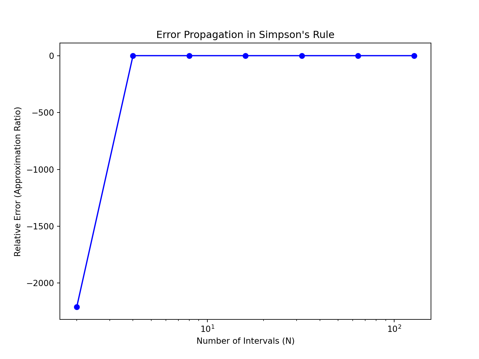

plt.figure(figsize=(8, 6))
plt.plot(N_values, ABSerrors, marker='o', linestyle='-', color='red')
plt.xscale('log')
#plt.yscale('log')
plt.xlabel('Number of Intervals (N)')
plt.ylabel('Absolute Error')
plt.grid(False)
plt.show()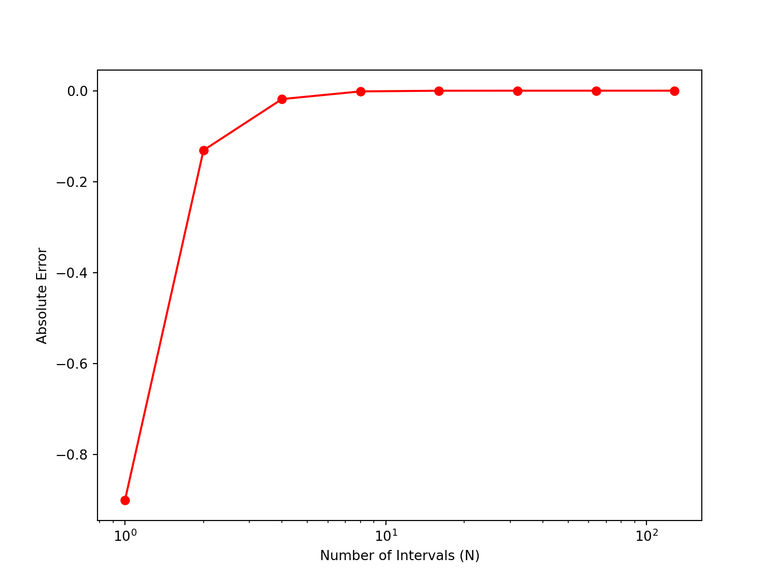

recreation of the breath cycle plot

P_in = np.zeros(1000)
P_ex = np.zeros(1000)
V = np.linspace(0.0,0.6,1000)

for i,x in enumerate(V):
  P_in[i] = fin(x)
  P_ex[i] = fex(x)

plt.clf()
plt.plot(V,P_in,V,P_ex)
plt.show()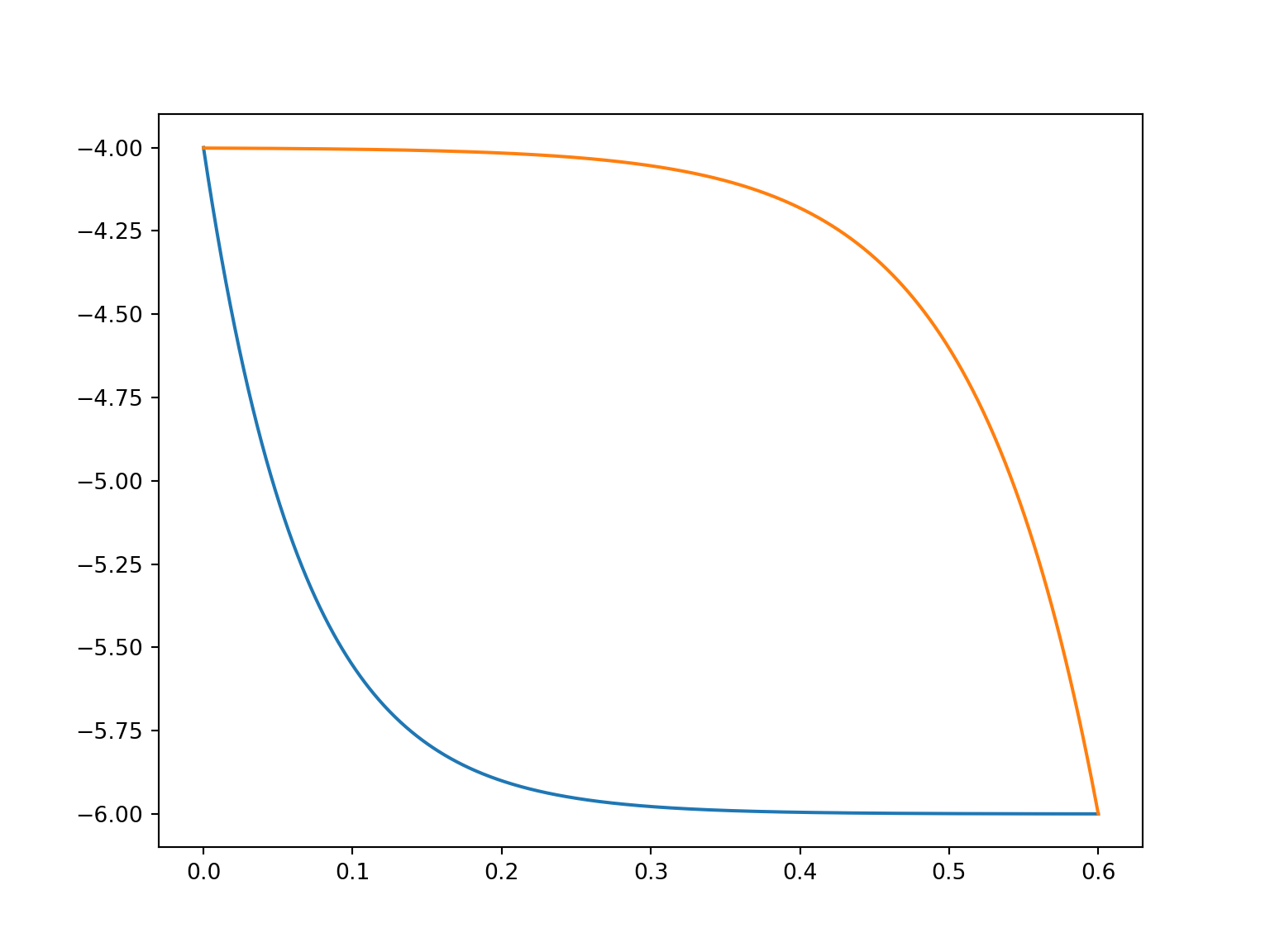

applied to the triple Integral

simpson(fx,0,1,100) * simpson(fy,0,1,100) * simpson(fz,0,1,100)

0.04166666666666682

f = lambda x,y,z : x**2 * y * z**3
simpson_value=np.prod(
  list(
    map(
      lambda I: simpson(I,0,1,100),
      [lambda x: f(x,1,1),lambda y : f(1,y,1),lambda z : f(1,1,z)]
      )
    )
  )

print(f'Simpson : {simpson_value:2.6f} \n Trapez : {trapez_value:2.6f}')

Simpson : 0.041667 
 Trapez : 0.041673

Check how fast Simpsons and the triagle Method converges

Number_of_iterations = [ 2**n for n in range(0,7) ]
f = lambda x : x**2  ; a = 0 ; b = 1 # true value I = 1/3 

for N in Number_of_iterations:
  err_trap = (trapez(f,a,b,N)-(1/3))
  err_simpson =  (simpson(f,a,b,N) -(1/3))
  print(f'{N} iterations:\n Trapez error {err_trap:2.5f}\n Simpson Error {err_simpson:2.5f}\n---')

1 iterations:
 Trapez error 0.16667
 Simpson Error 0.00000
---
2 iterations:
 Trapez error 0.04167
 Simpson Error 0.00000
---
4 iterations:
 Trapez error 0.01042
 Simpson Error 0.00000
---
8 iterations:
 Trapez error 0.00260
 Simpson Error 0.00000
---
16 iterations:
 Trapez error 0.00065
 Simpson Error 0.00000
---
32 iterations:
 Trapez error 0.00016
 Simpson Error 0.00000
---
64 iterations:
 Trapez error 0.00004
 Simpson Error 0.00000
---

Romberg integration Method

Function

def romberg(f,a,b,k,method):

  if method not in [simpson,trapez]:
    print("please define a valid method")
    return
  # init 
  #  For trapezoidal
  # estimates it is necessary to change the powers 4^j → 4^(j−1)
  q = 0 if method == simpson else 1   # q flag for method
  N_iter = np.array([(2**_) for _ in range(k)]) # number of iterations
  I = np.array([method(f,a,b,_) for _ in N_iter]) # first column of Integration matrix
  J = np.zeros((k,k))
  E = np.zeros((k,k))
  J[:,0] = I
  E[0,0] = 0
  
  for i in range(1,k):
    for j in range(1,i+1):
      J[i,j] = ((4**(j+q))*J[i,j-1] - J[i-1,j-1]) / ((4**(j+q))-1)
      E[i,j] = (J[i,j] - J[i-1,j]) / (4**(j+1+q) -1 )
  return J,E

Test

f = lambda x : x**2 + 10*x**3
J,E = romberg(f,0,10,5,simpson)
print(J)

[[33666.66666667     0.             0.             0.
      0.        ]
 [25333.33333333 22555.55555556     0.             0.
      0.        ]
 [25333.33333333 25333.33333333 25518.51851852     0.
      0.        ]
 [25333.33333333 25333.33333333 25333.33333333 25330.39388595
      0.        ]
 [25333.33333333 25333.33333333 25333.33333333 25333.33333333
  25333.34486058]]

print(E)

[[ 0.00000000e+00  0.00000000e+00  0.00000000e+00  0.00000000e+00
   0.00000000e+00]
 [ 0.00000000e+00  1.50370370e+03  0.00000000e+00  0.00000000e+00
   0.00000000e+00]
 [ 0.00000000e+00  1.85185185e+02  4.05055850e+02  0.00000000e+00
   0.00000000e+00]
 [ 0.00000000e+00  0.00000000e+00 -2.93944738e+00  9.93348780e+01
   0.00000000e+00]
 [ 0.00000000e+00  0.00000000e+00  0.00000000e+00  1.15272446e-02
   2.47637780e+01]]

Gauss–Legendre quadrature

Function of an integer approximationg pi

\[ \int_{-1}^{1} \frac{2}{1+x²}dx = \pi \]

steps:

Interpolate Integral to [-1,1] by mapping / scaling
choose N points
lookup coefs -> w,k
compute function on those points `

WeightsandAbscissae = {
  2: {
    "w": [1.0, 1.0],
    "x": [-0.5773502691896257, 0.5773502691896257]
    },
  3: {
    "w": [0.8888888888888888, 0.5555555555555556,0.5555555555555556],
    "x": [0.0, -0.7745966692414834,0.7745966692414834]
  },
  4: {
    "w": [0.6521451548625461, 0.6521451548625461,0.3478548451374538,0.3478548451374538],
    "x": [-0.3399810435848563, 0.3399810435848563,-0.8611363115940526,0.8611363115940526]
  },
  5: {
    "w": [0.5688888888888889, 0.4786286704993665,0.4786286704993665,0.2369268850561891,0.2369268850561891],
    "x": [0.0, -0.5384693101056831,0.5384693101056831,-0.9061798459386640,0.9061798459386640]
  },
  6: {
    "w": [0.3607615730481386, 0.3607615730481386,0.4679139345726910,0.4679139345726910,0.1713244923791704,0.1713244923791704],
    "x": [0.6612093864662645, -0.6612093864662645,-0.2386191860831969,0.2386191860831969,-0.9324695142031521,0.9324695142031521]
  }
}

WeightsandAbscissae[2]["w"]

[1.0, 1.0]

WeightsandAbscissae[2]["x"]

[-0.5773502691896257, 0.5773502691896257]

def Gaussq(f,a,b,N):
  # linear transformation
  alpha = (b-a)/2
  beta = (a+b)/2
  
  # obtain w and x
  w = WeightsandAbscissae[N]["w"]
  x = WeightsandAbscissae[N]["x"]
  
  # initialize I
  I = 0
  
  # Applying the n n point Gaussian quadrature 
  for i in range(N):
    I += alpha * w[i] * f( (alpha*x[i]+beta) ) 
    
    
  return I


f = lambda x : 2/(1+x**2)
Gaussq(f,-1,1,6)- np.pi

-0.0001292389556466489

Brute Force itegration in two dimensions

rectangle enclosing the circle


f = lambda x,y : 2*((x**2)*y*np.exp(-0.1*((x-1))**2+y**2 + 2*(x-2)*(y-1)))
ax = -1; bx= 2
ay = 0; by = 4
dx = 0.01; dy = dx

I = 0 

for x in np.arange(ax+dx/2,bx,dx):
  for y in np.arange(ay+dy/2,by,dy):
      I = I + f(x,y) * dx *dy

print(f'The integral is {I}')

The integral is 4836458.586055034

f = lambda x,y : 2*((x**2)*y*np.exp(-0.1*((x-1))**2+y**2 + 2*(x-2)*(y-1)))



ax = -1; bx= 2
ay = 0; by = 4
dx = 0.01; dy = dx

I = 0 

for x in np.arange(0,10,dx):
  for y in np.arange(0,10,dy):
    # check domain
      if x**2+y**2 <= 2**2:   
        I = I + f(x,y) * dx *dy

print(f'The integral is {I}')

The integral is 12.002988414109822

poission integral


f = lambda x,y : np.exp(-(x**2+y**2))    # possion integral
dx = 0.01
dy = dx
I = 0 

for x in np.arange(-4,4,dx):
  for y in np.arange(-4,4,dy):
    # check domain
      if x**2+y**2 < 3**2:   
        I = I + f(x,y) * dx *dy

print(f'The integral is {I}\nError: {I-np.pi} ')

The integral is 3.141204302200772
Error: -0.0003883513890210466

Euler Derivation


def eulerderiv(y0,f,t0,tf,N):
    h = (tf-t0) / N # define
    t_vec = [t0]
    y_vec = [y0]
    f_vec = [f(y0)]

    for t in range(1,N): # for each interval
        t_vec.append(t0 + t*h)
        y = []
        for j in range(len(y0)): # for each variable of f (ie len of y0)
            y.append(y_vec[t-1][j] + f_vec[t-1][j]*h)

        y_vec.append(y)
        f_vec.append(f(y_vec[t]))

    return t_vec, y_vec


def eulernp(y0,f,a,b,N):
    # define interval size h:
    h = (b-a) / N

    # pre allocate Y vector dim = N x y0:
    Y = np.zeros((N,y0.shape[0])); Y[0] = y0 # -> set y0 to first pos in Y vec

    # differentiate using euler's method:
    for t in range(1,N):
         Y[t] = Y[t-1] + f(Y[t-1])*h

    # calculate timeframe directly:
    dT = np.linspace(a, b, N)

    return dT, Y

f = lambda x : np.array([x[1], 0-x[0]*40**2])
# phi = 0
###
tf = 1
t0 = 0
y0 = np.array([5,0])
N = 1000

dT, F = eulernp(y0,f,t0,tf,N)

plt.plot(dT, [x[0]for x in F])
plt.show()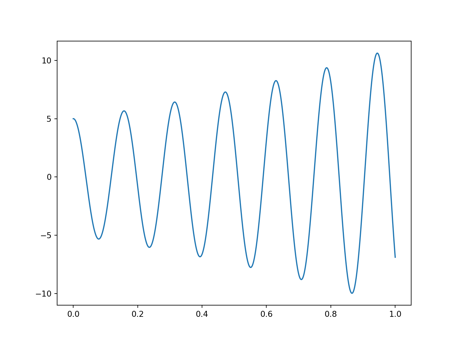

runge kutta 4th

def rungekutta4(y0,f,a,b,N):

    h = (b-a) / N # define interval size h

    Y = np.zeros((N,y0.shape[0]))
    Y[0] = y0
    F = np.zeros((N,y0.shape[0]))
    F[0] = f(a,Y[0])

    for t in range(1, N):
        k1 = h * f(a + (t-1)*h,         F[t-1])
        k2 = h * f(a + (t-1+0.5)*h,     F[t-1] + 0.5*k1)
        k3 = h * f(a + (t-1+0.5)*h,     F[t-1] + 0.5*k2)
        k4 = h * f(a + t*h,             F[t-1] + k3)

        F[t] = F[t-1] + (k1 + 2 * k2 + 2 * k3 + k4) / 6
        Y[t] = F[t]

    dT = np.linspace(a, b, N)

    return dT, Y,F

### 4

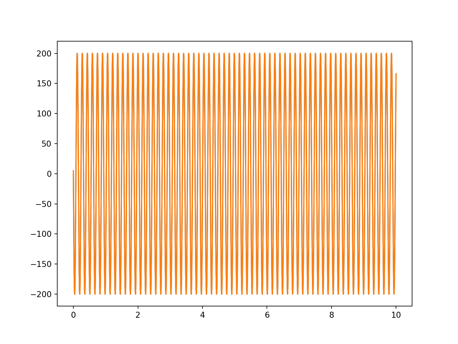
# The equation that describes the position of a harmonic oscillator is, ¨x + ω2x = 0,
# where ω = 40 is the angular frequency of oscillation, (the frequency is f = ω2π ).

# define function f with two arguments sice runge kutta needs a t argument

f = lambda t,x : np.array([x[1], 0-x[0]*40**2])


tf = 10
t0 = 0
y0 = np.array([5,0])
N = 10000

dT, Y,F = rungekutta4(y0,f,t0,tf,N)


plt.plot(dT,[x[0]for x in F],dT,[x[0]for x in Y])

plt.show()

#### 5

# The number of bacteria, N (t), present in a certain medium depends on the amount
# of nutrients available, g(t). These quantities vary with time according to the equa-
# tions

Shooting Method

Partial differential equations